FPGA-based graph neural network accelerator solution

GNN has very high requirements for computing power and storage, and the software implementation efficiency of its algorithm is very low. Therefore, the industry has a very urgent need for hardware acceleration of GNN. Although there are many solutions for traditional convolutional neural network (CNN) hardware acceleration, hardware acceleration of GNN has not been fully discussed and studied. At the time of writing this white paper, neither Google nor Baidu could search for Chinese research materials on GNN hardware acceleration. The motivation for writing this white paper is to combine the latest foreign GNN algorithms, research on acceleration technology, and discussion of GNN acceleration technology based on field programmable logic gate arrays (FPGA), and present it to readers in the form of an overview. The

Introduction to Graph Neural Network (GNN)

At the macro level, the architecture of GNN has many similarities with traditional CNN, such as convolutional layer, pooling, activation function, machine learning processor (MLP), fully connected layer (FC layer) and other modules, which can all be applied to GNN. The figure below shows a relatively simple GNN architecture.

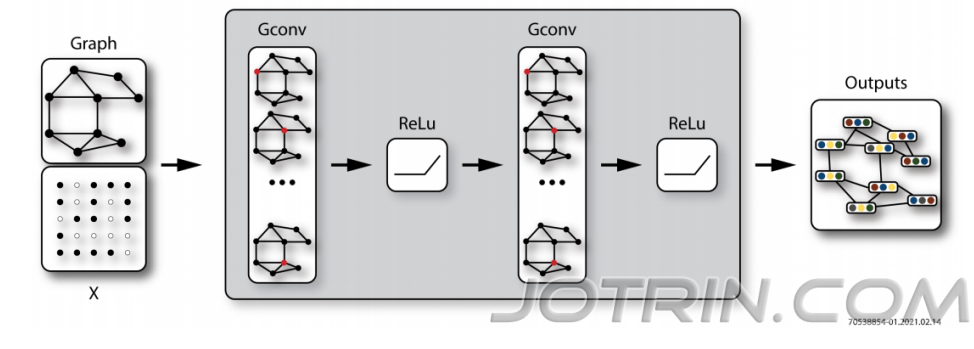
Figure 1: Typical GNN architecture

However, the convolution calculation of graphics data in GNN is different from the two-dimensional convolution calculation in traditional CNN. As an example in the figure below, the convolution calculation process of the red target node is as follows:

1. Graph convolution - uses the nearest neighbor function to sample the features of surrounding nodes and calculate the average. The number of adjacent nodes is uncertain and disordered (non-Euclidean data)

2. Two-dimensional convolution - Use the convolution kernel to sample the features of surrounding nodes and calculate the weighted average. The number of adjacent nodes is determined and ordered (Euclidean data)

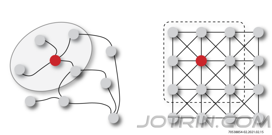
Figure 2: Graph convolution and two-dimensional convolution

Introduction to the GraphSAGE algorithm

The academic community has conducted a lot of research and discussion on the GNN algorithm and proposed many innovative implementation methods. Among them, GraphSAGE, proposed by Stanford University in 2017, is an inductive representation learning algorithm used to predict dynamic, new, and unknown node types in large-scale graphs. It is also specially optimized for graphs with a large number of nodes and rich node features. As shown in the figure below, the calculation process of the GraphSAGE algorithm can be divided into three main steps:

1. Adjacent node sampling - used to reduce complexity, generally sampling two layers, sampling several nodes in each layer.

2. Aggregation - used to embed the target node, that is, a low-dimensional vector representation of the graph.

3. Prediction - Use embedding as input to the fully connected layer to predict the label of target node d.

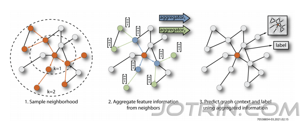
Figure 3: Visual representation of the GraphSAGE algorithm

1.Sample neighborhood

1. Sample neighborhood

2.Aggregate feature informaTIon from neighbors

2. Aggregate feature information from neighbors

3.Predict graph context and label using aggregated informaTIon

3. Use aggregated information to predict graphic conditions and labels

In order to implement GraphSAGE algorithm acceleration in FPGA, its mathematical model must be understood in order to map the algorithm to different logic modules. The code shown below illustrates the mathematics of this algorithm. In order to solve this problem,

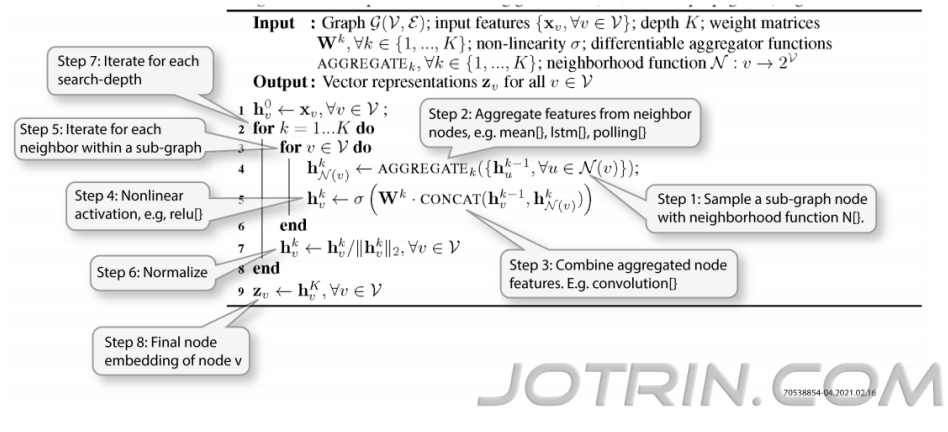
Figure 4: Mathematical model of the GraphSAGE algorithm

Step 1： Sample a sub-graph node with neighborhood funcTIon N［}。

Step 1: Use the nearest neighbor function N［} to sample the subgraph nodes.

Step 2： Aggregate features from neighbor nodes， e.g. mean［}， lstm［}， polling［}

Step 2: Aggregate the features of adjacent nodes, such as mean［}, lstm［}, polling］

Step3： Combine aggregated node features. E.g. convoluTIon［}

Step 3: Merge the aggregated node features. For example convolution [}

Step 4： Nonlinear activation， e.g， relu［}

Step 4: Non-linear activation, such as relu [}

Step 5： Iterate for each neighbor with a sub-graph

Step 5: Iterate each neighborhood using subgraph

Step 6： Normalize

Step 6: Normalization

Step 7： Iterate for each search-depth

Step 7: Iterate for each depth search

Step 8： Final node embedding of node v

Step 8: Final node embedding of node v

For each target node xv to be processed, the GraphSAGE algorithm will perform the following operations:

1. Sample nodes in the subgraph through the nearest neighbor sampling function N(v).

2. Aggregate features of adjacent nodes to be sampled. The aggregate function can be mean(), lstm() or polling(), etc.

3. Merge the aggregation result with the output representation of the previous iteration and perform convolution using Wk.

4. Perform nonlinear processing on the convolution results.

5. Iterate multiple times to end the processing of all adjacent nodes of the current kth layer.

6. Standardize the results of the k-th layer iteration.

7. Multiple iterations to end the processing of all K layer sampling depths.

8. Embed the final iteration result zv into the input node xv.

GNN accelerator design

GNN algorithm involves a large number of matrix calculations and storage access operations. The efficiency of running this algorithm on traditional x86 architecture servers is very low, manifested by slow speed and high energy consumption.

new graphics processor (GPU) can significantly improve the calculation speed and energy efficiency ratio of GNN. However, GPUs have shortcomings in storage scalability, making them unable to handle the massive number of nodes in the graph. The way GPU instructions are executed can also lead to excessive computational latency and uncertainty; therefore, it is not suitable for scenarios that require real-time computing graphics.

The various design challenges mentioned above make the industry urgently need a GNN acceleration solution that can support high concurrency, real-time computing, have huge storage capacity and bandwidth, and can be extended to data centers.

GNN accelerator based on FPGA design scheme

Achronix's Speedster® 7t family of FPGA products (and the first device in the family, the AC7t1500), are high-performance FPGA devices optimized for data center and machine learning workloads, eliminating several performance bottlenecks that exist in central processing unit (CPU), GPU and traditional FPGA-based solutions. Speedster7t series FPGA products use TSMC's 7nm FinFET process. Its architecture uses a revolutionary new two-dimensional network-on-chip (NoC), an original machine learning processor matrix (MLP), and adopts a high-bandwidth GDDR6 controller, 400G Ethernet and PCI Express Gen5 interface. While ensuring ASIC-level performance, it provides users with flexible hardware programmability. The figure below shows the architecture of the high-performance FPGA device Speedster7t1500.

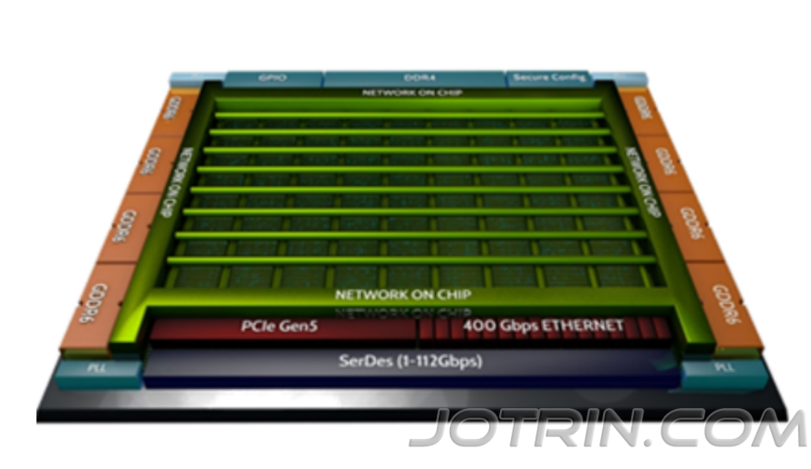
Figure 5: Architecture of Achronix high-performance FPGA device Speedster AC7t1500

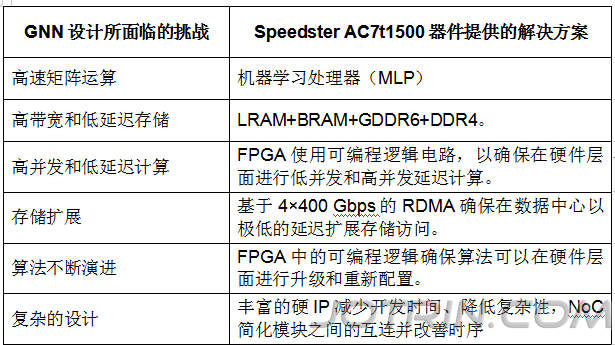
The above features make the Achronix Speedster7t1500 device a perfect solution to the various challenges faced in GNN accelerator design.

Table 1: Challenges faced by GNN design and solutions provided by Achronix Speedster7t1500 FPGA device

GNN accelerator top-level architecture

This GNN accelerator is designed for the GraphSAGE algorithm, but its design can also be applied to other similar GNN algorithm acceleration. Its top-level architecture is shown in the figure below.

Figure 6: Top-level architecture of GNN accelerator

Synthesizable IPs

Synthesizable IP

GNN Core： Preforms GNN computation

GNN kernel: performing GNN calculations Challenges faced by

RoCE-Lite： Memory scalability with RDMA

RoCE-Lite: Storage scalability with RDMA

Harden IPs

Hardened IP

NoC： High speed and unified IP connectivity

NoC: High-speed, unified IP connectivity

DDR4 Ctrl： Large memory for graph storage

DDR4 Ctrl: Large storage capacity for graphics storage Part 1ABE043850009 produced by

GDDR6 Ctrl： High speed memory for computing

GDDR6 Ctrl: High-speed storage for computing

PCIe Gen5×16： High throughout host interface

PCIe Gen5×16: High-throughput host interface

Ethernet 400GE： High speed network

Ethernet 400GE: High-speed Network

The architecture consists of the following modules:

• žThe GNN kernel in the picture is the core part of the algorithm implementation (details below).

• žRoCE-Lite is a lightweight version of the RDMA protocol for remote storage access over high-speed Ethernet to support graph computing of massive nodes.

• ž400GE Ethernet controller is used to carry RoCE-Lite protocol.

• žGDDR6 memory is used to store high-speed access data required during GNN processing (DDR4 as backup large-capacity memory). This memory is used to store data with relatively low access frequency, such as graphics data to be preprocessed.

• žPCIe Gen5 ×16 interface provides a high-speed host interface for data interaction with server software.

All the above modules are interconnected through NoC with high bandwidth.

GNN kernel microarchitecture

Before starting to discuss the microarchitecture of the GNN kernel, it is necessary to review the GraphSAGE algorithm. The aggregation and merging of its inner loops (including convolutions) account for most of the algorithm's computational and storage accesses. Through research, we derived the characteristics of these two steps, which are as follows.

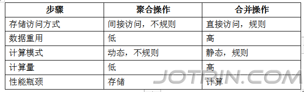
Table 2: Comparison of aggregation and merging operations in GNN algorithm

It can be seen that aggregation operations and merge operations have completely different requirements in terms of computing and storage access patterns. Aggregation operations involve sampling of neighboring nodes. However, a graph is a non-Euclidean data type - its size and dimensions are undefined and unordered, its matrices are sparse, and its node locations are random. As a result, storage access is irregular and data reuse is difficult.

In the merge operation, the input data are the aggregation result (a low-dimensional representation of the nodes) and the weight matrix. Its size and dimensions are fixed, with linear storage locations. So there is no challenge for storage access, but the matrix is ​​very computationally intensive.

Based on the above analysis, we decided to choose to use two different hardware structures in the GNN core accelerator design to handle the aggregation and merging operations respectively (as shown in the figure below):

• žAggregator - Sampling and aggregating graph adjacent nodes via an array of Single Instruction Multiple Data (SIMD) processors. A single instruction can be predefined as mean() average calculation, or other applicable aggregation function; multi-data means that a single mean() mean calculation requires feature data of multiple adjacent nodes as input, and these data come from the subgraph sampler. The SIMD processor array is load balanced through the scheduler Agg Scheduler. The adjacency matrix and node feature data h0v read back from GDDR6 or DDR4 by the subgraph sampler through the NoC are cached in the adjacency list buffer (Adjacent List Buffer) and the node feature buffer (Node Feature Buffer) respectively. The result of aggregation hkN(v) is stored in the aggregation buffer (Aggregation Buffer).

• žCombiner - convolves the aggregation results through the systolic matrix PE. The convolution kernel is the Wk weight matrix. The convolution results are processed nonlinearly by the ReLU activation function and are also stored in the Partial Sum Buffer for the next iteration.

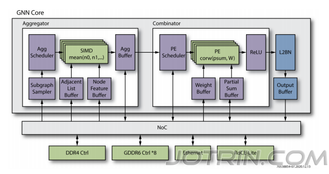
Figure 7: GNN kernel functional block diagram

After the merged result is standardized by L2BN, it is the final node representation hkv. In a typical node classification prediction application, the node representation hkv can obtain the classification label of the node through a fully connected layer (FC). This process is one of the traditional machine learning processing methods, which is not reflected in the GraphSAGE literature, and this function is not included in this architecture.